Module 1 - Integrated Decision Units (IDUs) for Land Use Suitability Modeling#

1. Introduction#

“Land units, or land-mapping units, are areas with and qualities that differ sufficiently from those of other land units to affect their suitability for different land uses.”

As suggested by the title, the workshop deals with creating Integrated Decision Units (IDUs), a vector geographic data represented in polygons. Two major applications of IDU includes:

demarcation of a tract of land into smaller (homogeneous) parcels
creation of (mapping) units for geospatial analysis

We introduce a technical solution for creating IDUs in QGIS. We will begin by introducing the conceptual framework IDU is based on; then, moving onto QGIS functions that are involved in the particular solution; and, finally, looking at an example of the THLD District in Ghana.

2. Datasets Description#

The homogeneity of an IDU is determined by land properties or attributes, such as soil, land cover, slope, elevation, etc. Therefore, these information should be utilized in the creation of IDUs. As to which specific ones to use, it is often a combined result of data availability and the spatial scale of the particular question at hand. In general, the more datasets are involved in the process of creating IDUs the more complicated (in terms of granularity) the IDU system will be. In this workshop, we used two datasets: (1) land cover and (2) soil drainage.

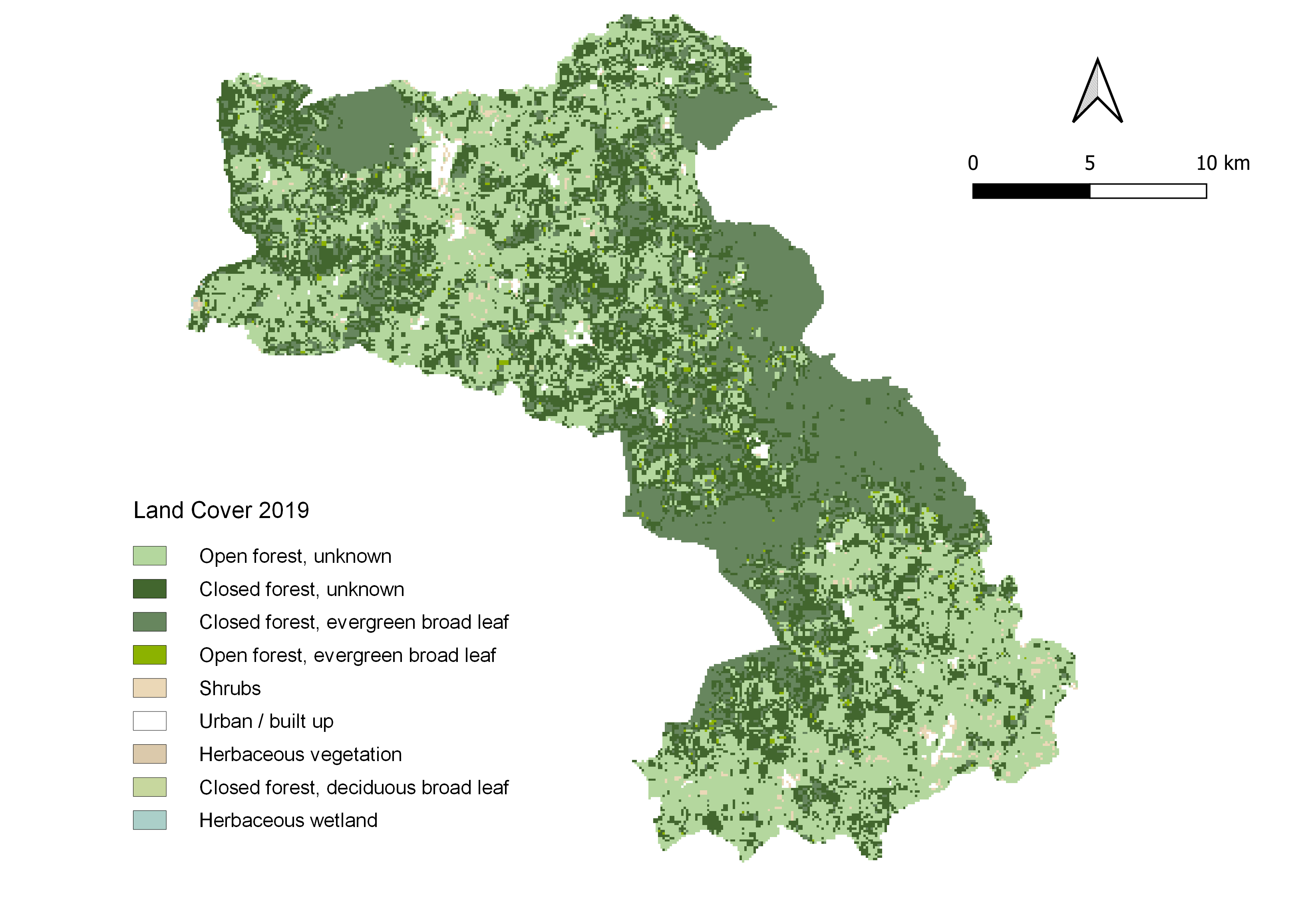
Land Cover

Land cover is used because it reflects the condition of the land surface, which is directly related to the potential land use. For example, when developing a new town, land that is classified as "closed forest" would require more labor than land that is "open forest." Therefore, it is useful to consider land cover when creating IDUs.

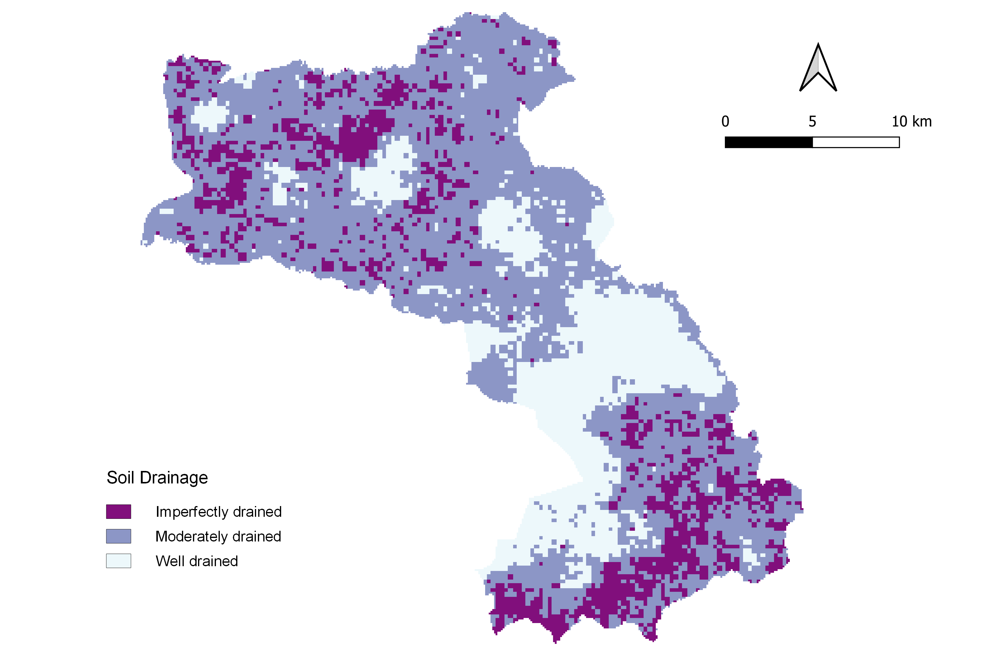
Soil Drainage

Soil drainage is used because it reflect the permeability of the land surface in natural conditions, which usually indicative to the landform and environmental characteristics of the land.

🔔 Download and Use the Datasets

The datasets can be found at here. It is organized by two Districts Assembly of Ghana, namely Asante Akim Central (AAC) District and Twifo-Hemang Lower Denkyira (THLD) District. THLD datasets are used as examples in the following training materials, whereas AAC datasets will be used for the exercise. To download the datasets, simply click here, which will download the entire GALUP repository as a zip file. Unzip the downloaded file and navigate to the appropriate location to use the datasets.

ID	File Name	Data Format	Type	Description
1	gas_station.shp	vector	point	Gas station locations in Ghana

3. Key Functions#

The table below shows all of the tools used in this module. You can find out more information about each tool by following the attached link. Later, we will take a more in depth look at 6 functions that are key to this workflow.

Raster Analysis	Vector Analysis	Conversion	Selection
Raster calculator	Eliminate selected polygons	Rasterize	Extract by attribute
Reclassify by table	v.clean	r.to.vect	Select by expression
Proximity	Merge vector layers	Raster pixels to points
r.null	Subdivide	Multipart to singleparts
	DBSCAN clustering	Fix geometries

3.1 DBSCAN clustering#

For Defined distance (DBSCAN), if the Minimum Features per Cluster can be found within the Search Distance from a particular point, that point will be marked as a core-point and included in a cluster, along with all points within the core-distance. A border-point is a point that is within the search distance of a core-point but does not itself have the minimum number of features within the search distance. Each resulting cluster is composed of core-points and border-points, where core-points tend to fall in the middle of the cluster and border-points fall on the exterior. If a point does not have the minimum number of features within the search distance and is not a within the search distance of another core-point (in other words, it is neither a core-point nor a border-point), it is marked as a noise point and not included in any cluster.

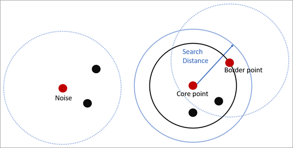Fig. 2 How DBSCAN is calculated. Source: ESRI.

Usage: This tool is used to detect areas where points are concentrated and where they are separated by areas that are empty or sparse. Points that are not part of a cluster are labeled as noise. The results from running the DBSCAN algorithm help us identify points that make up a cluster and points that are noise.
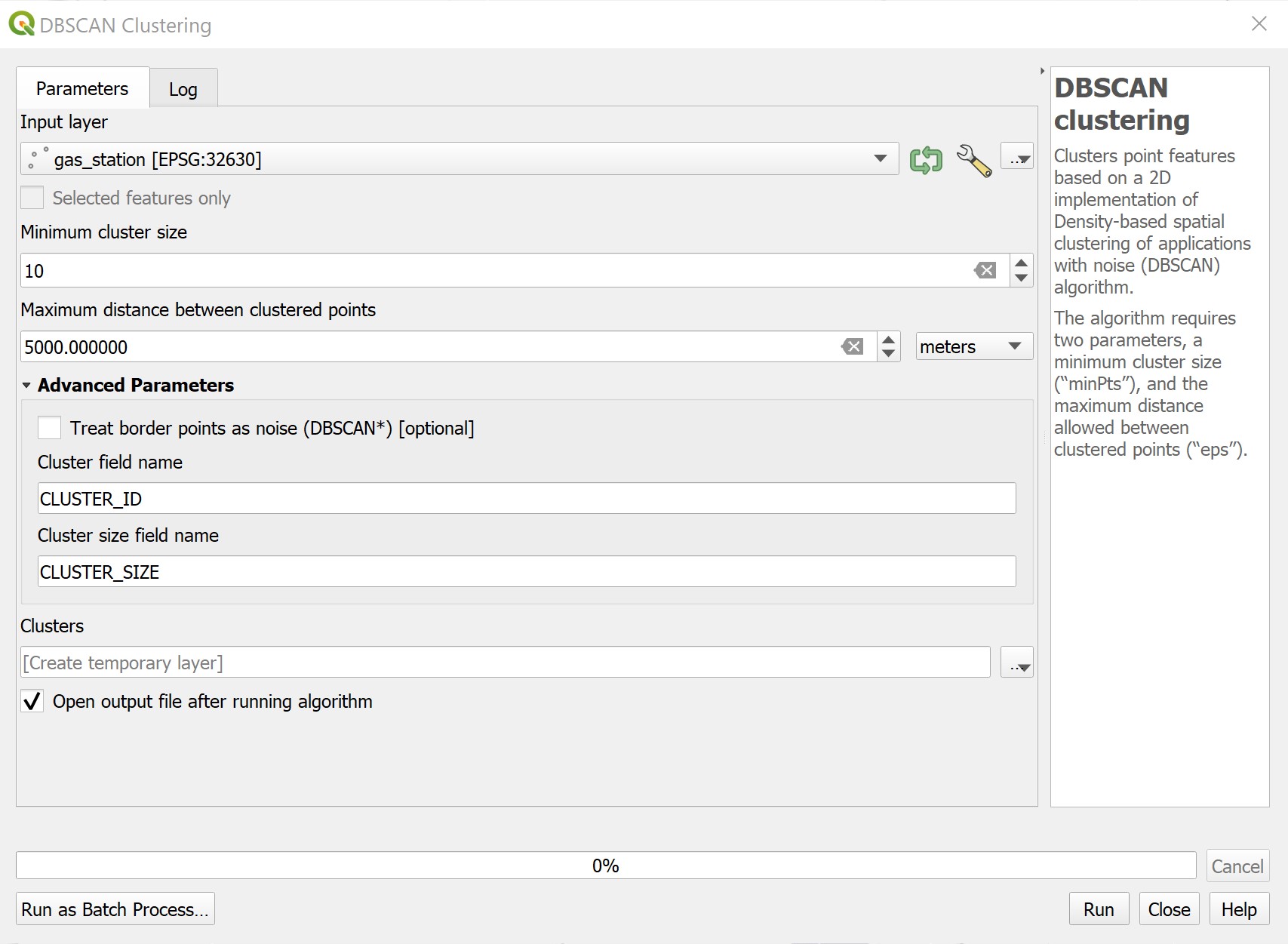
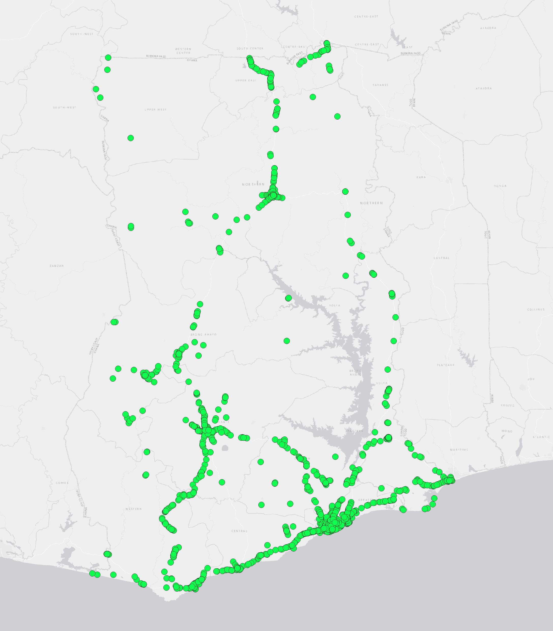
Example: As an example, we will use DBSCAN clustering to identify clusters of gas stations within Ghana. The datasets used are listed below:

ID	File Name	Data Format	Type	Description
1	gas_station.shp	vector	point	Gas station locations in Ghana

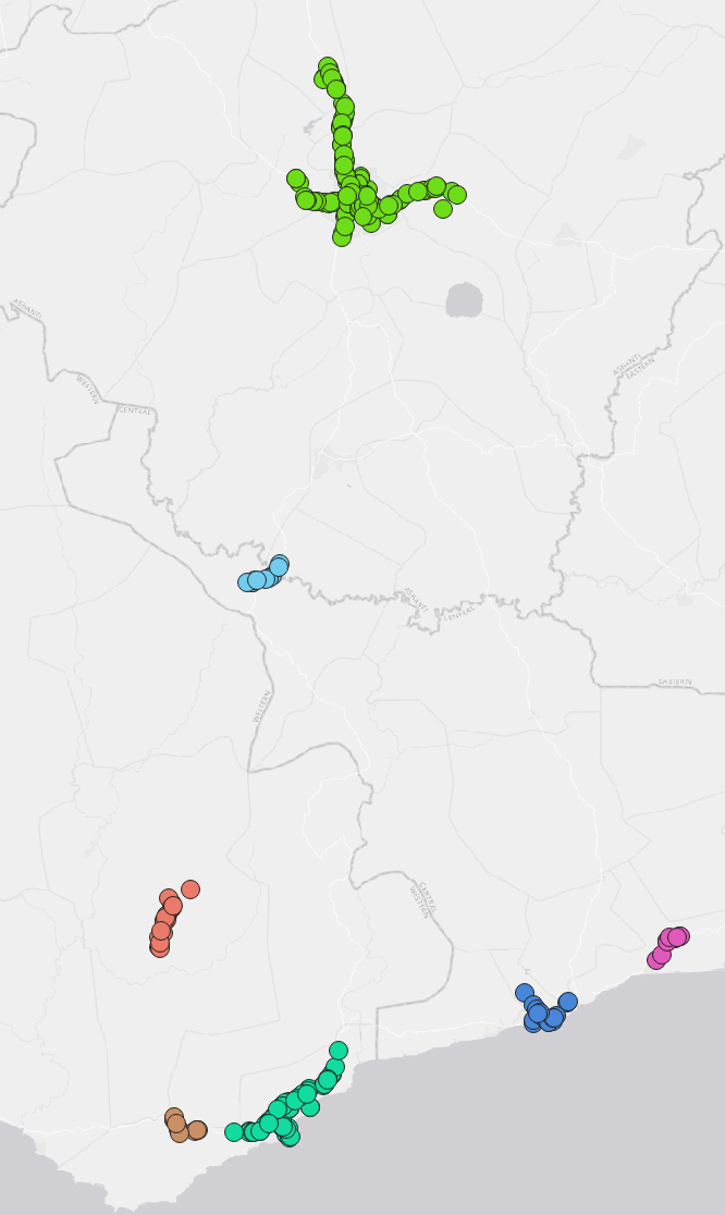
The two figures below display the parameter settings and the output of the tool.

Parameter Settings	Input	Output

3.2 Proximity#

The Proximity tool calculates the Euclidean distance from the center of the source cell to the center of each of the surrounding cells. Conceptually, the Euclidean algorithm works as follows: for each cell, the distance to each source cell is determined by calculating the hypotenuse with x_max and y_max as the other two legs of the triangle. This calculation derives the true Euclidean distance, rather than the cell distance. The shortest distance to a source is determined, and if it is less than the specified maximum distance, the value is assigned to the cell location on the output raster.

Determining true Euclidean distance. Source: ESRI

Usage: This tool gives the measured Euclidean distance from every cell to the nearest source. The distances are measured in the projection units of the raster, such as feet or meters, and are measured from cell center to cell center.

📌 The projected units of a raster layer can be found under the information tab in the layer properties

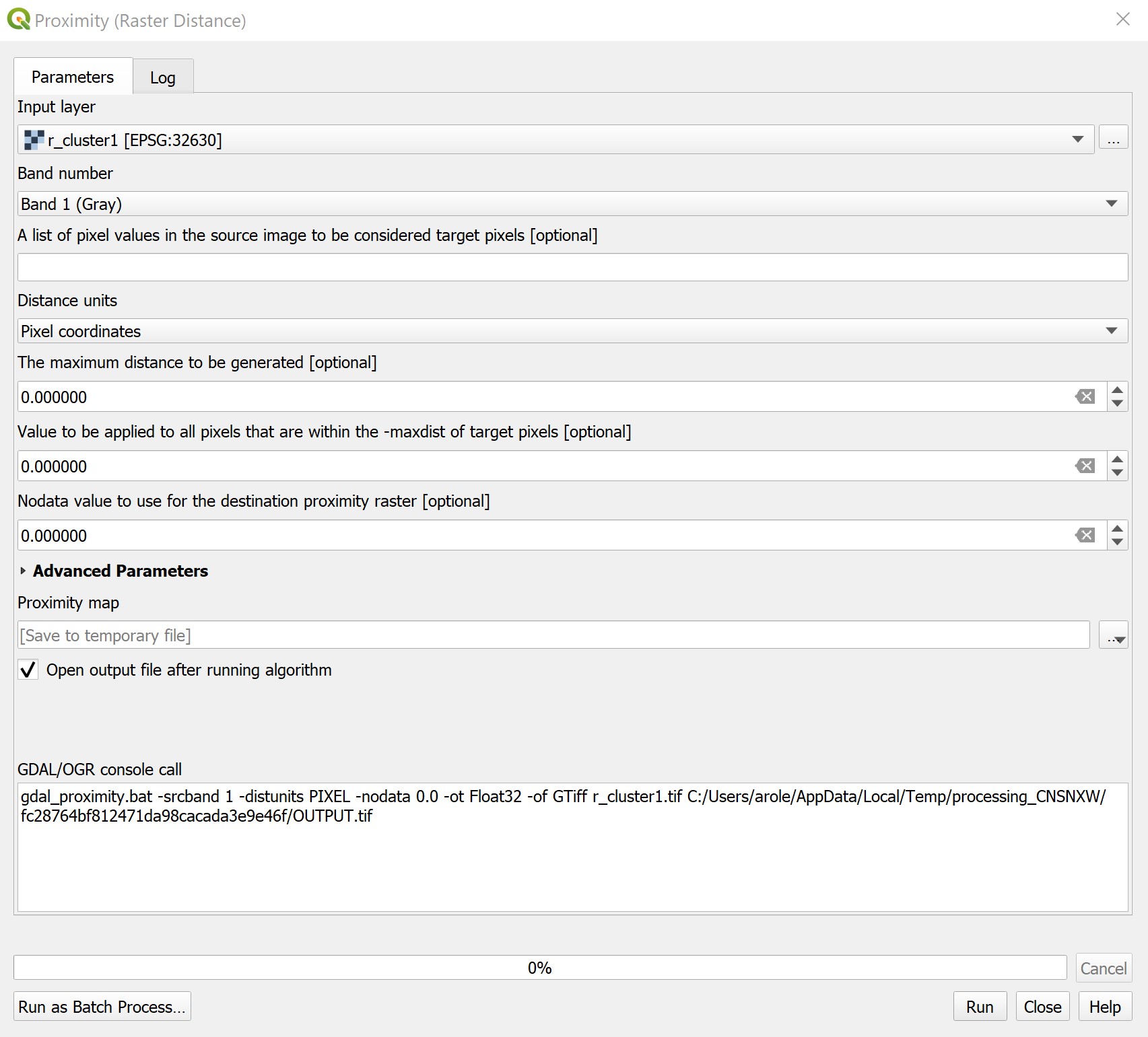
Example: Now we will use the Proximity tool in order to determine the Euclidean distance from a gas station cluster to the rest of the raster cells.

ID	File Name	Data Format	Description
1	r_cluster1.tif	raster	Cluster 1 in raster format

The two figures below illustrate the parameters and output of the Proximity tool.

Parameter Settings	Output

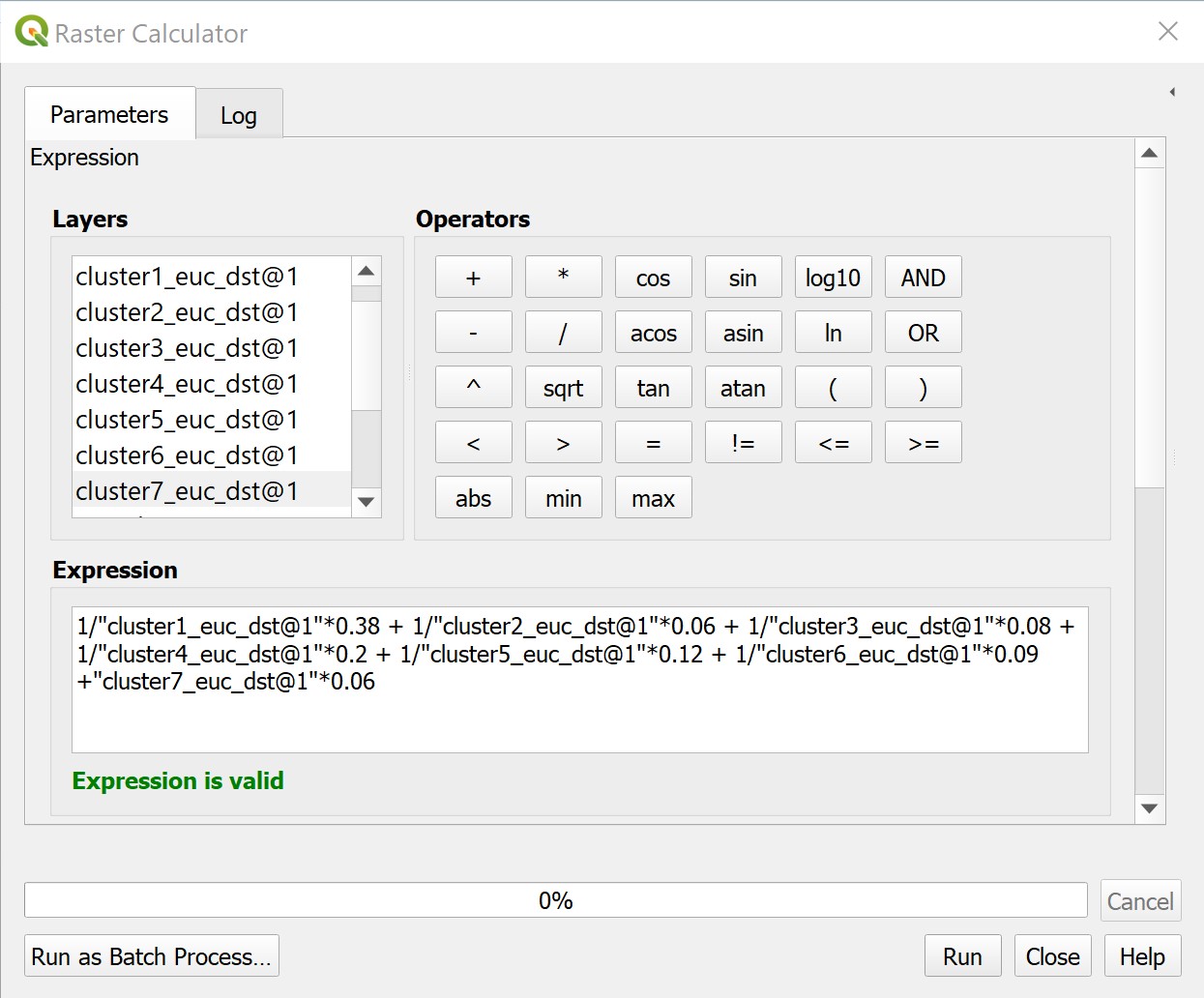
3.3 Raster Calculator#

The Raster calculator tool allows you to create and execute Map Algebra expression that will output a raster. We will be using a distance decay model in order to assign weights to each cluster. Distance decay, also known as the Gravity Model or the Inverse Square Law, is the tendency of a spatial relationship between one place and another to weaken as the distance between them increases³.

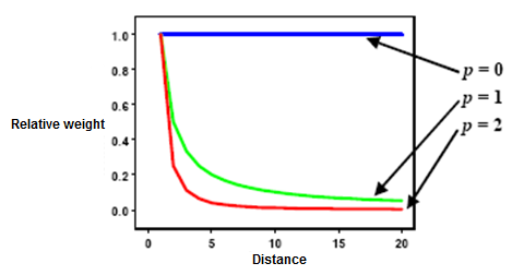Fig. 2 How DBSCAN is calculated. Source: ESRI.

Usage: The Raster calculator tool is used to individually weight and multiply proximity rasters together.

The weighting formula that we will use is: w * 1/distance.

Where w is equal to the number of points (urban pixels) in a cluster divided by the total number of points in all clusters.

Here is what our full equation looks like:
Example:

ID	File Name	Data Format	Description
1	cluster1_euc_dst.tif	raster	Euclidean distance from cluster 1
2	cluster2_euc_dst.tif	raster	Euclidean distance from cluster 2
3	cluster3_euc_dst.tif	raster	Euclidean distance from cluster 3
4	cluster4_euc_dst.tif	raster	Euclidean distance from cluster 4
5	cluster5_euc_dst.tif	raster	Euclidean distance from cluster 5
6	cluster6_euc_dst.tif	raster	Euclidean distance from cluster 6
7	cluster7_euc_dst.tif	raster	Euclidean distance from cluster 7

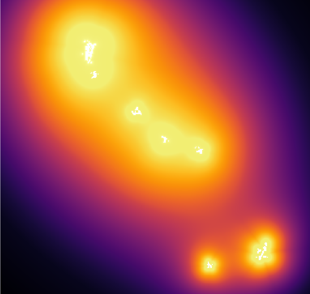
The figures below show the parameters and output of the Raster calculator tool.

Parameter Settings	Output

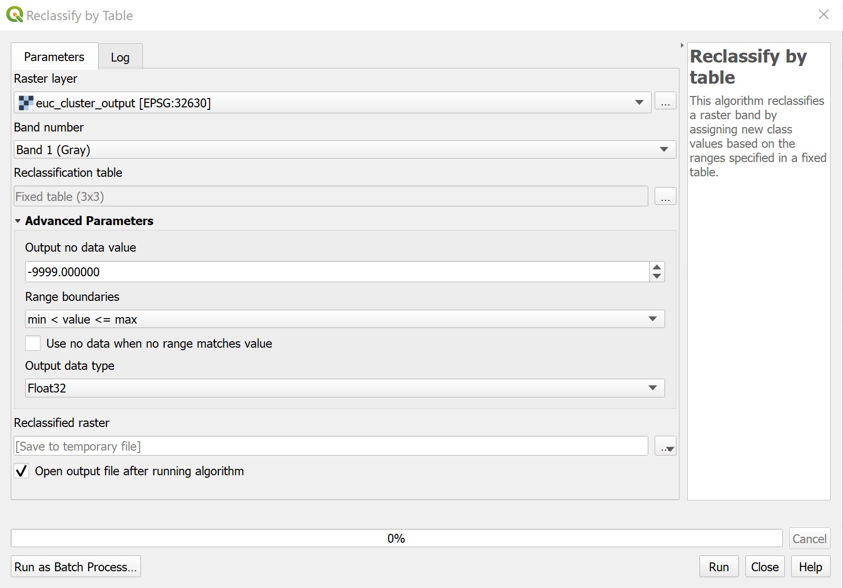
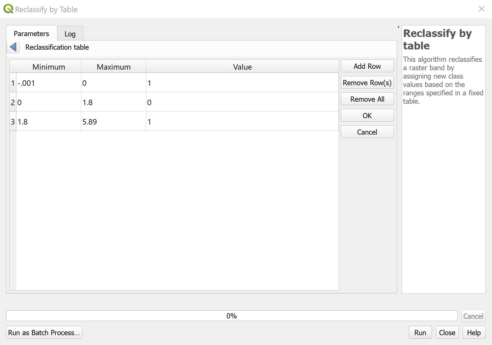
3.4 Reclassify by Table#

Reclassify by table is a tool that reclassifies a raster band by assigning new class values based on ranges specified in a fixed table.

Usage: This tool is used to reclassify raster values.
Example:

ID	File Name	Data Format	Description
1	euc_cluster_output.tif	raster	Result of adding together the weighted clusters 1 and 2

The figures below show the parameters and output for the Reclassify by table tool.

📌 Check the details of an image:
If you can’t see the image clearly, click on the image to view it in a new page, which will show the image in its original size.

Parameter Settings	Table Parameters	Output

📌 Here is a helpful strategy: If you want to keep track of what raster cells are combined when multiplying raster layers together, try reclassifying the raster values as prime numbers. The product of two prime numbers can only be the result of those specific numbers, allowing you to identify what cells were combined.

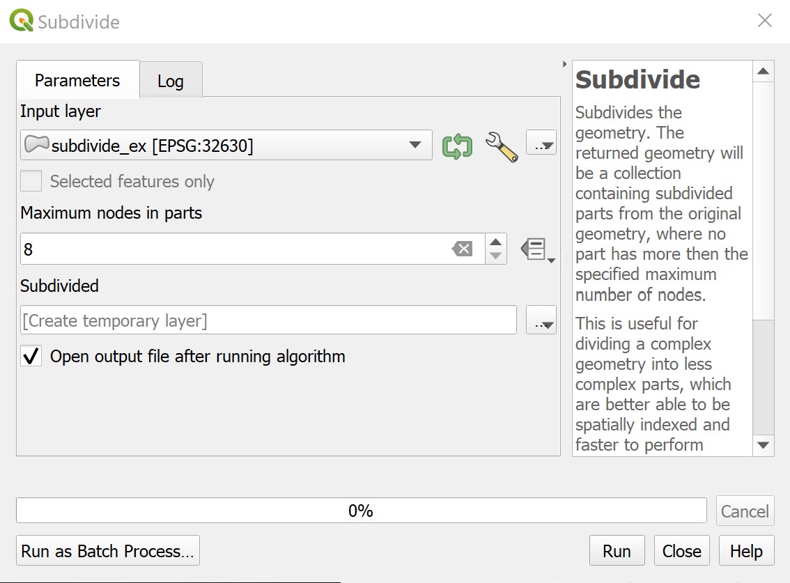
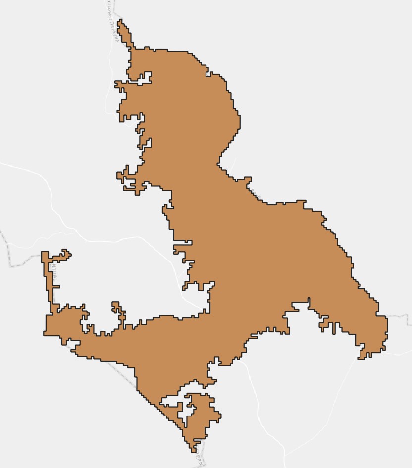
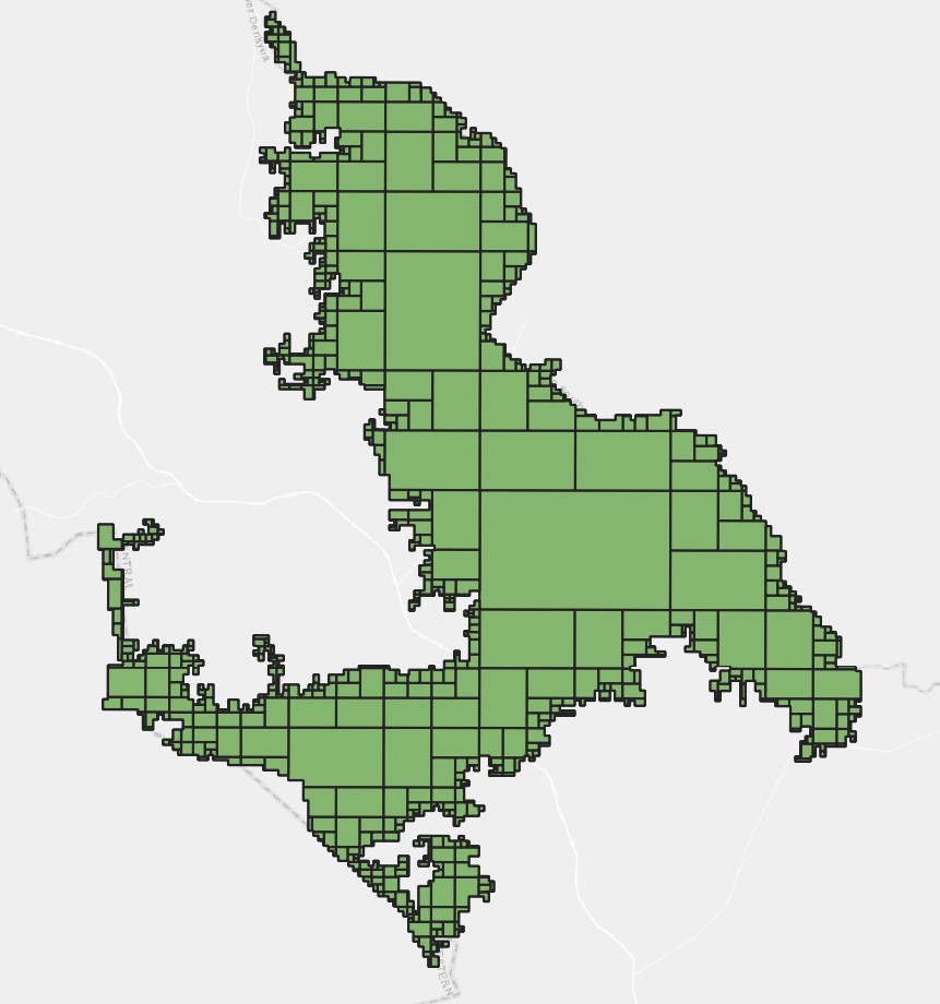
3.5 Subdivide#

Subdivide is a tool that subdivides the original geometry into smaller parts, where no part has more than the specified maximum number of nodes.

Usage: The subdivide tool is used to break down complex geometries into more manageable parts. In our case, this tool allows us to subdivide large areas of land into IDUs.
Example:

ID	File Name	Data Format	Type	Description
1	subdivide_ex.shp	vector	polygon	Geographic area to be subdivided

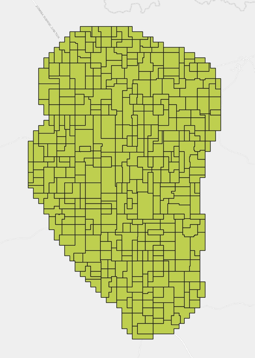
The figures below show the parameters and output for the Subdivide tool.

Parameter Settings	Input	Output

3.6 Eliminate Selected Polygons#

Eliminate selected polygons is a tool that combines selected polygons by erasing the common boundary with nearby polygons. The merge can be based on largest common boundary, largest area or smallest area.

Usage: Eliminate selected polygons is used to refine the IDUs by eliminating sliver polygons and other irregularities.
Example

ID	File Name	Data Format	Type	Description
1	eliminate_ex.shp	vector	polygon	Input polygons to be eliminated

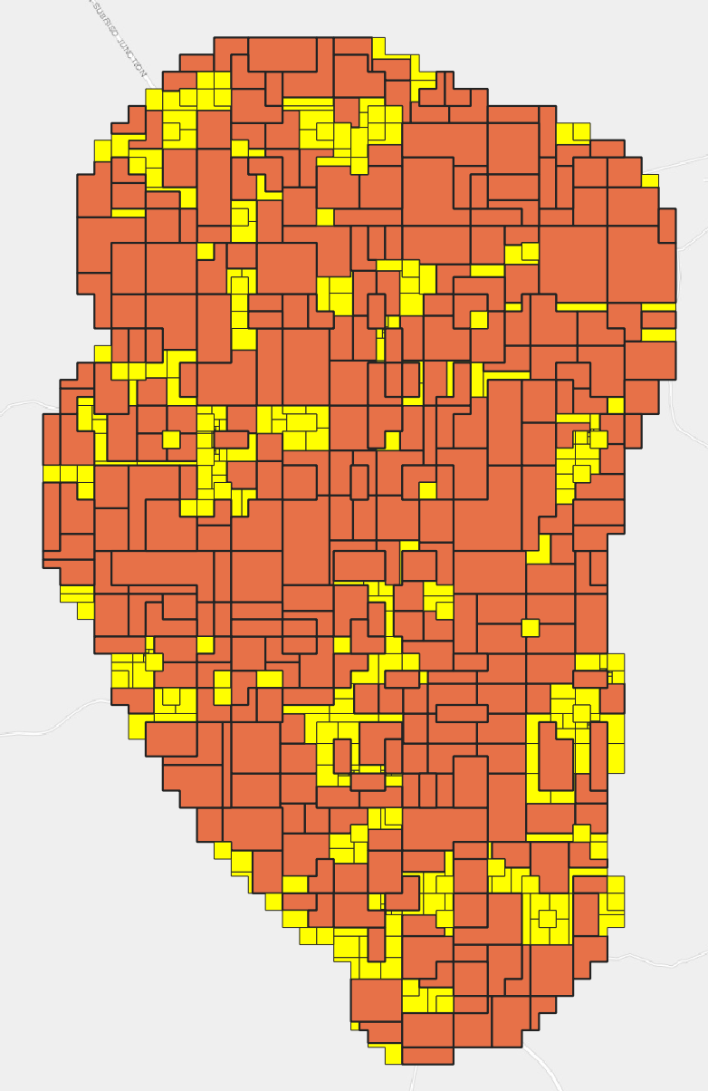
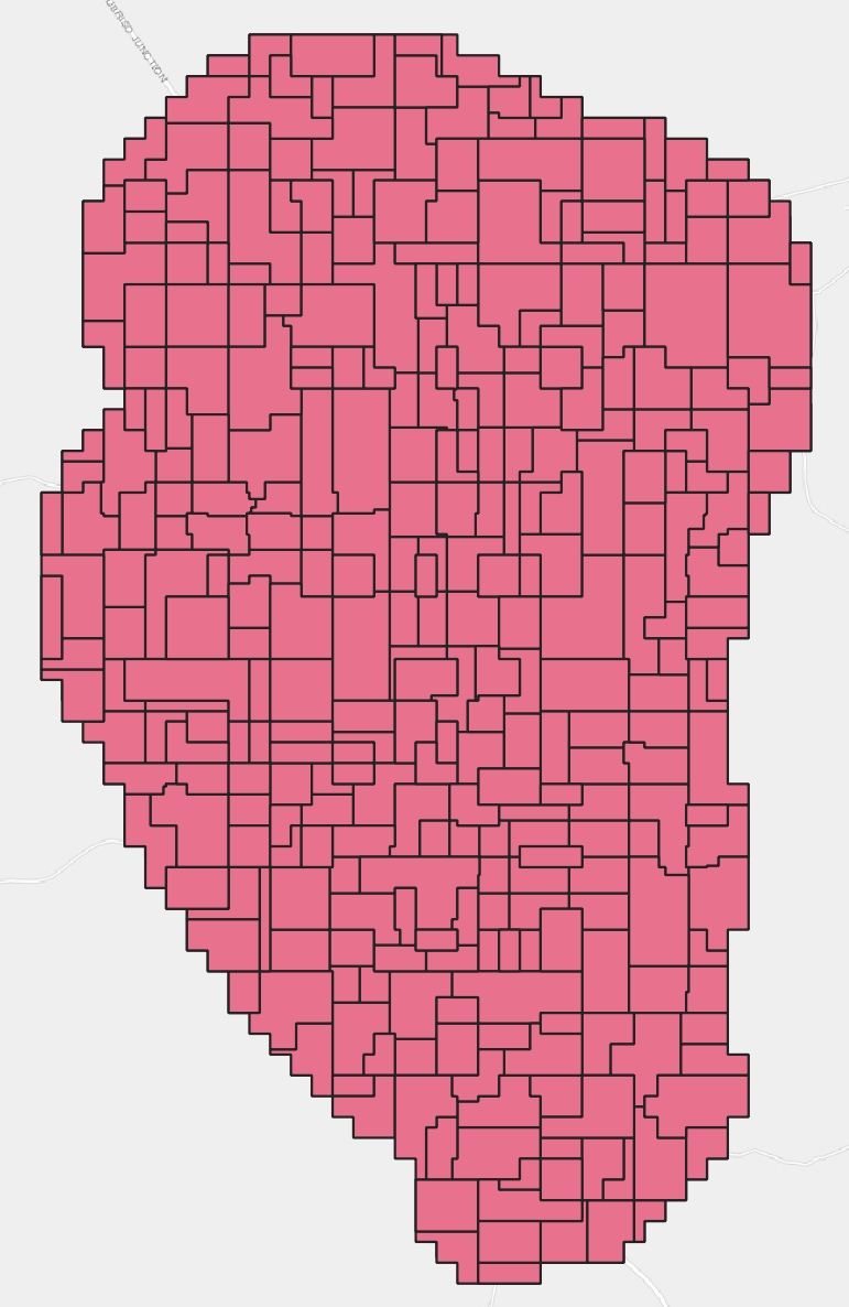
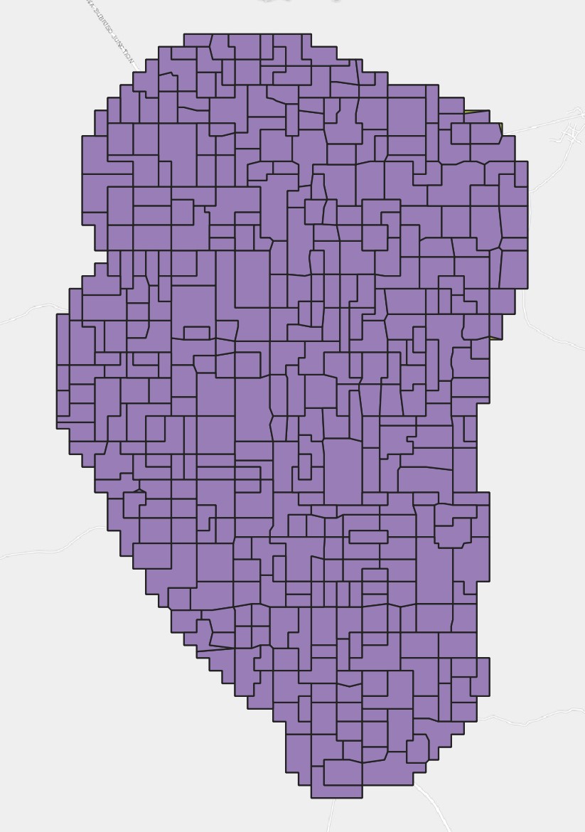
The figures below show the parameters for the Eliminate selected polygons tool.

Parameter Settings	Input	Output

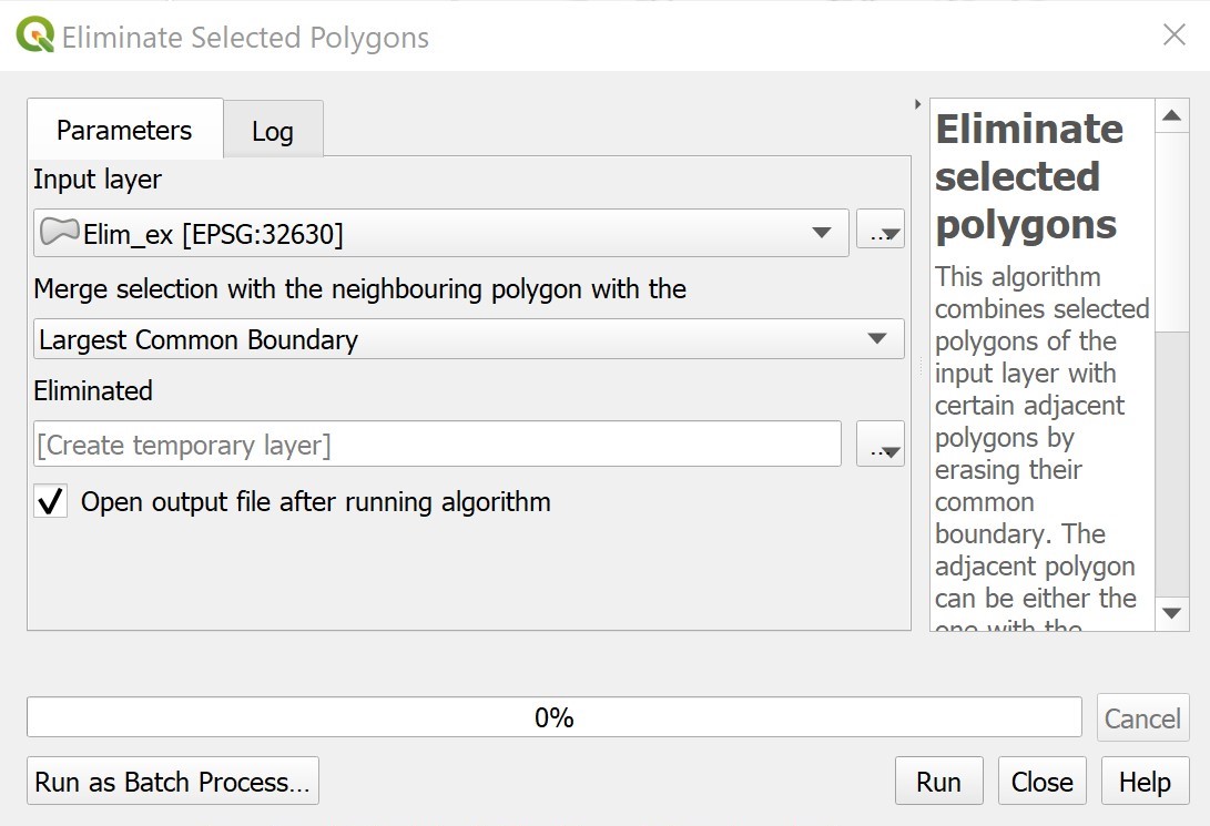
📌 Note: This workflow utilized largest common boundary as the parameter for Eliminate selected polygons because this gave us the best result. Try using the other methods for merging with the neighboring polygons to see which gives you the best result.

3.7 v.clean#

v.clean is a tool that cleans input layers using a selection of tools. The table below shows what tools are available:

v.clean
break	snap	rmdangle	chdangle	rmbridge
chbridge	rmdupl	rmdac	bpol	prune
rmarea	rmline	rmsa

There is also an optional parameter called Input feature type which allows you to specify what you want to be cleaned. This makes the v.clean tool more effective. The table below shows the possible input feature types:

v.clean
area	point	line	boundary
centroid	face	kernel

Usage: The v.clean tool is used for making each of the IDUs more regularly shaped. We will be utilizing all of the tools to clean our feature type, which is area.
Example:

ID	File Name	Data Format	Type	Description
1	clean_ex.shp	vector	polygon	Input polygon to be cleaned

The figures below show the parameters and output for the v.clean tool.

Parameter Settings	Input	Output

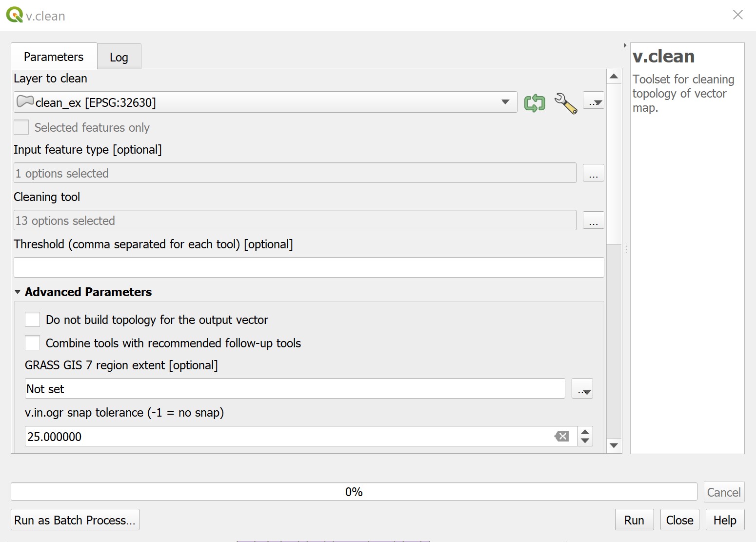
📌 Note: In order for this tool to work, you must specify a location for the output shapefile to be saved.

4. The QGIS Workflow of Creating IDUs#

The diagrams below show the general process of the IDU workflow.

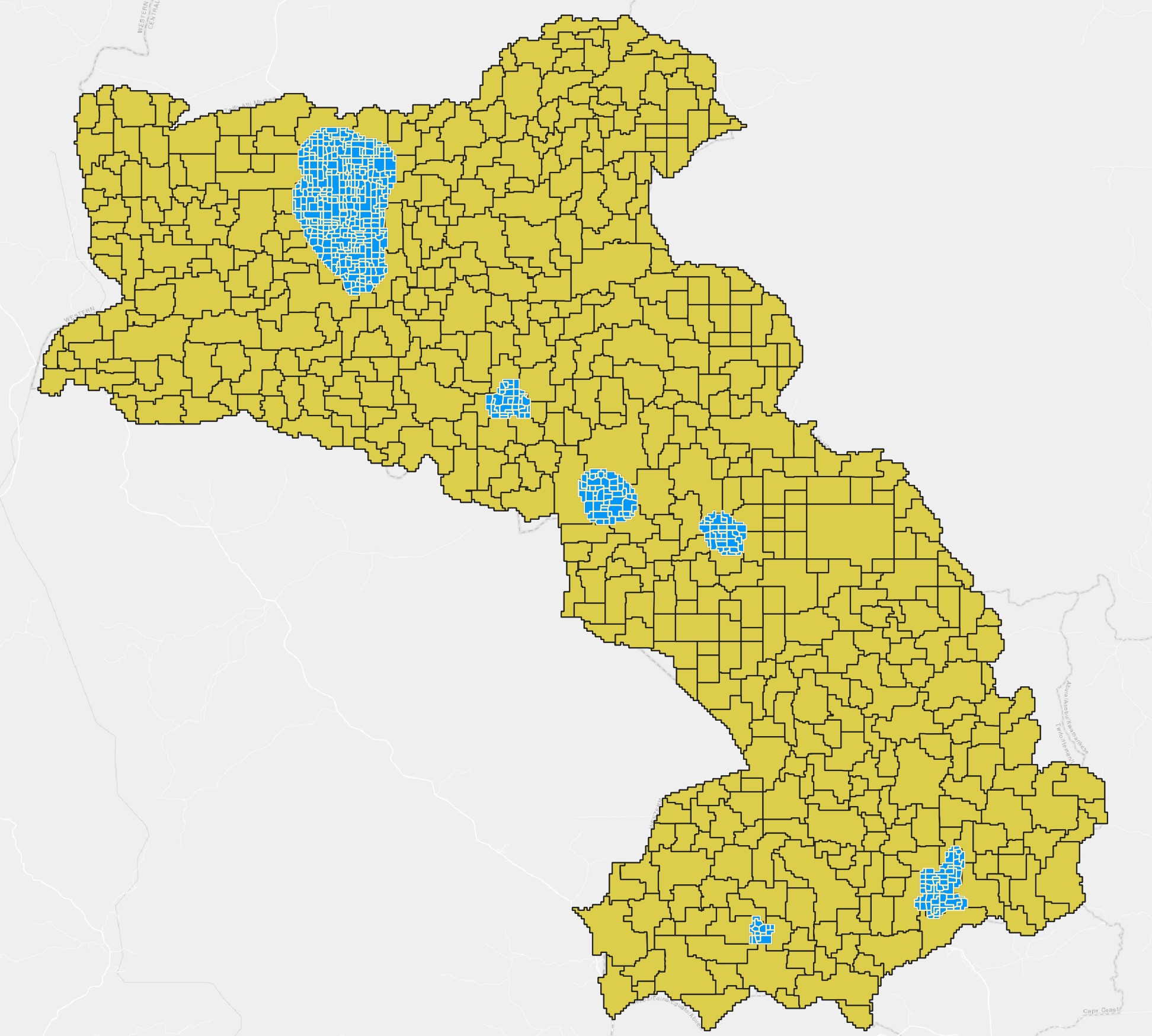
4.1 Developing urban clusters#

The first part of the IDU workflow focuses on developing urban clusters and distinguishing the boundary between these clusters and the rest of the THLD District. This can be done through a series of 4 geoprocessing steps: identify urban clusters, measure distance to each cluster, aggregate inverse distance raster, and define urban boundary.

In order to identify urban clusters, urban areas of the THLD District must first be extracted from the base land use raster. This was done by converting the land use raster to vector points and then extracting points according to their land use designation. Points designated with land use type 6 make up the urban areas that we are looking for. Once these have been extracted, they are entered into the DBSCAN clustering tool.The output from the DBSCAN tool is our urban clusters.
Now that DBSCAN has identified urban clusters, each of these clusters must individually be extracted, converted to raster, and then processed using the proximity tool.
After completing the previous steps, we can move on to calculating the area of influence for each cluster. This influence is calculated by dividing the number of points in a cluster by the total number of points for all clusters. These are now weighted using the inverse distance formula, where 1 is divided by the proximity raster and multiplied by the weight.
To define the boundary between the urban and rural areas of the THLD District, we can reclassify our weighted raster. This reclassified raster will be binary, where 1 corresponds to the urban area and 0 corresponds to the rural area.

Developing urban clusters

IDU part 1 video demo (click to watch)

💡 A quick note on the Reclassification table

The output raster generated by multiplying proximity rasters and their respective weights is monotonically increasing. In other words, there are no 0 values at the center of an urban cluster. Therefore, the "Reclassification table" shown at about "07:30" of the video demo can be simplified with only two classes as:

Minimum Maximum Value

0 0.0039 0

0.0039 1 1

Minimum	Maximum	Value
0	0.0039	0
0.0039	1	1

IDU in-depth explanation: Calculating Urban Clusters (click to watch)

4.2 Calculating IDUs#

The second part of the IDU workflow focuses on the actual calculating of the IDUs. This can be done by performing the following 4 geoprocessing functions: overlay input rasters, separate rural and urban areas, process vector data (iteration) and merge results.

The first step in calculating the IDUs is to create the base suitability raster. In order to make the calculations easier, we are going to reclassify the land cover raster into three general categories Once this is done, the generalized land cover and drainage rasters are ready to be combined. In order to combine these rasters, they must first be reclassified as prime numbers. The reason we do this is to keep track of what raster values are combined when we multiply the land cover and drainage rasters together (for further explanation on why we use prime numbers, you can refer back to section 3.3 Raster Calculator). After the layers are reclassified, they are multiplied together using raster calculator.
Next, the combined suitability raster needs to be separated into urban and rural areas. This is where we use the urban and rural rasters that were calculated in the first part of the IDU workflow. The combined raster is multiplied by the urban and rural rasters, respectively. This calculation maintains the suitability of the targeted area while setting the rest of the raster equal to 0. After this is done for both the urban and rural rasters, the r.null tool is used to convert the 0 raster values to No Data.
With the urban and rural parts of the suitability raster separated, it is time to create the first iteration of the IDUs. Starting with either the urban or rural suitability rasters, r.to.vect is used to convert the raster layer to a vector layer. The fix geometries tool is then used on the vector layer, creating a valid input for the subdivide tool.The subdivide tool returns a multipart polygon which must be converted to a single part polygon before further processing. At this point, the subdivided areas are very small and irregular. This is addressed by eliminating very small polygons and merging them with other nearby, larger polygons. Multiple iterations are required in order to create regular, consistent IDUs.
Once the IDUs have been established, all that is left to do is some final cleaning (if you choose) and to merge the urban and rural layers back together. The v.clean tool is used to make the IDUs more regularly shaped. This change is very subtle and is not required if you feel that your IDUs are regular enough already. The urban IDUs and rural IDUs can then be merged to create the final IDU layer.

Calculating IDUs

The GIS process described above leads us to the final IDUs of THLD district. It is worth noting that the output may not be identical or 100% reproducible due to the fact that there are multiple iterative processes involved and Here, one output is presented in the map below (click to expand). The output shapefile is also provided and can be found at here. You can locate the file in the downloaded zip file of this GitHub repository and visualize it in QGIS.

IDU part 2 video demo (click to watch)

IDU in-depth explanation: Weight clusters and create urban/rural masks (click to watch)

IDU part 3 video demo (click to watch)

IDU in-depth explanation: Iterative elimination and v.clean tool (click to watch)

💡 A quick note on the parameters used in the demo
It is important to understand that the parameters used in this demo is based on the fact that the raster cell size is 100 meters. For example, in the Select by expression tool, 10000 (approx.) is used to select polygons that will be eliminated because that is the area of a single cell in the original raster is 10,000 square meters (i.e., 100 x 100). One must adjust the parameter when a different cell size is in question. A parameter of 10,000 is certainly not at the right magnitude for a raster with cell size of 10 meters.

THLD final IDU map

5. Exercise and Post-training Survey#

Please complete this Exercise.
Please submit your exercise here.
Please take this post-training survey (required).

Reference#

Buchhorn, M., Lesiv, M., Tsendbazar, N.-E., Herold, M., Bertels, L., & Smets, B. (2020). Copernicus Global Land Cover Layers—Collection 2. Remote Sensing, 12(6). https://doi.org/10.3390/rs12061044
Hengl, T., Heuvelink, G. B. M., Kempen, B., Leenaars, J. G. B., Walsh, M. G., Shepherd, K. D., Sila, A., MacMillan, R. A., De Jesus, J. M., Tamene, L., & Tondoh, J. E. (2015). Mapping Soil Properties of Africa at 250 m Resolution: Random Forests Significantly Improve Current Predictions. PLOS ONE, 10(6), e0125814. https://doi.org/10.1371/JOURNAL.PONE.0125814
de Smith, M. J., Goodchild, M. F., & Longley, P. A. (2018). Geospatial analysis: A comprehensive guide to principles, techniques and software tools (6th ed.). https://www.spatialanalysisonline.com/HTML/index.html