Module 1 - Time Series Analysis#

Instructor: Dr. Aditya Singh (aditya01@ufl.edu)
Co-authors: Silas Achidago (s.achidago@ufl.edu) and Julie Peeling (juliepeeling@ufl.edu)

What will you learn from this module?

Time Series Analysis Concept and Fundamentals
Time Series Analysis Methods
Techniques for Time Series Analysis in GEE (Google Earth Engine)

1. Introduction to Time Series Analysis#

Geospatial Time series analysis techniques help monitor and quantify landscape changes across time and space. Mapping temporal changes provides information on the impact of urbanization, land degradation, phenology, and environmental parameter trends like rainfall and temperature.

Common Applications of Time Series Analysis:

Identifying urban expansion,
Mapping deforestation,
Monitoring flood or fire-related damage,
Indentifying regions experiencing changes in temperature or precipitation.

_{Landcover changes for Greater Accra Metropolitan Area (GAMA) from the year 1991 to 2015.

(Source)}

2. Basics of Time Series Analysis#

Spatial/geospatial data is information on the location, shape, and extent of objects in a geographic space represented as points, paths, areas, or surfaces.
Temporal data are data that represent the state of a particular object at a given point of time. Temporal data collected over several intervals create time-series data.
Spatio-temporal data are data that describe the state of objects or processes across both space and time.

_{MODIS EVI and NDVI (Source)}

Using Remote Sensing to Conduct Time Series Analysis:

In the context of remote sensing, time series analysis allows us to measure and quantify changes in spatio-temporal processes from space.
For effective monitoring to occur, data needs to: 1) have suitable spatial and spectral resolution to detect the phenomena, and 2) have a frequent-enough repeat interval to detect change.
Assuming the object is detectable using a specific sensor, the timing of acquisition needs to be tuned to the rate of the process being studied. For example, discrete event detections (such as floods or fires) can be conducted by collecting images before and after that event has occurred. Images need to be closely spaced in time for assessing rapidly changing phenomena, such as vegetation greenup after rain. For monitoring long-term changes, data can be aggregated over the time domain of interest, and then assessed on annual or monthly basis (urban expansion, temperature rise, etc.).
The availability of satellite data over different spatio-temporal resolutions therefore limits the kinds of proceses that can be studied.
Some trends may need to be decomposed into their underlying components for generating insights into the dynamics. For example, temperature usually has a strong seasonal component in addition to potentially annual components in some regions.

Types of Time Series Analysis

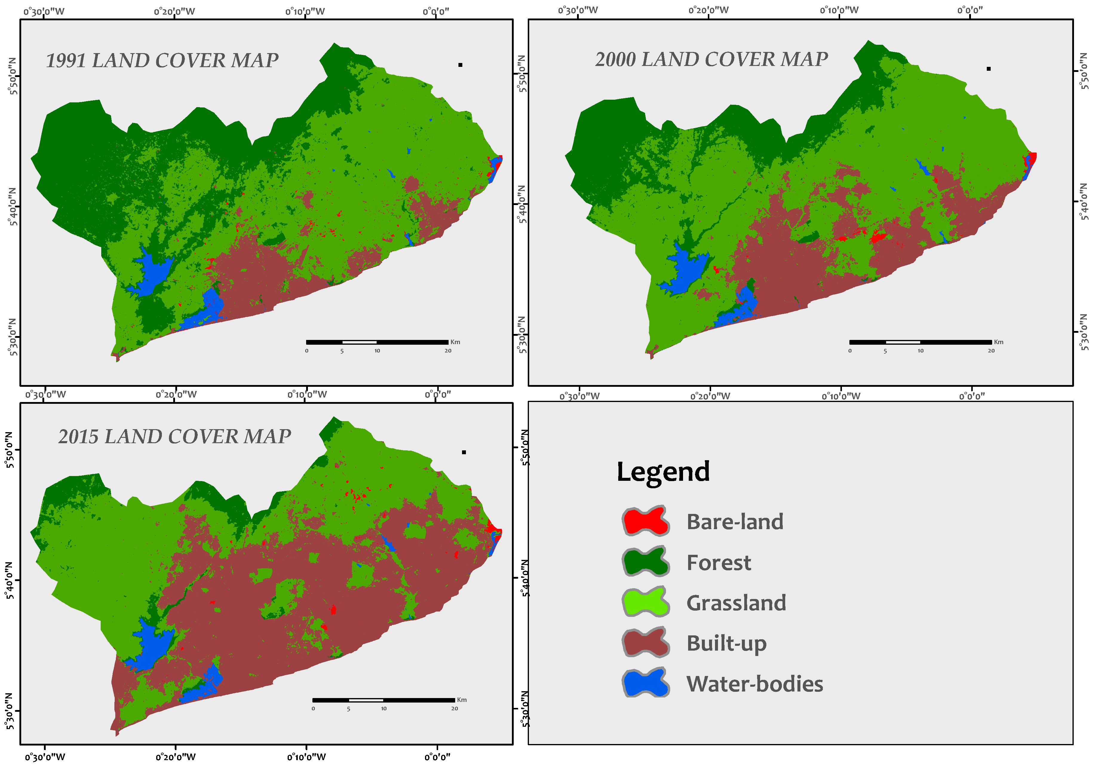
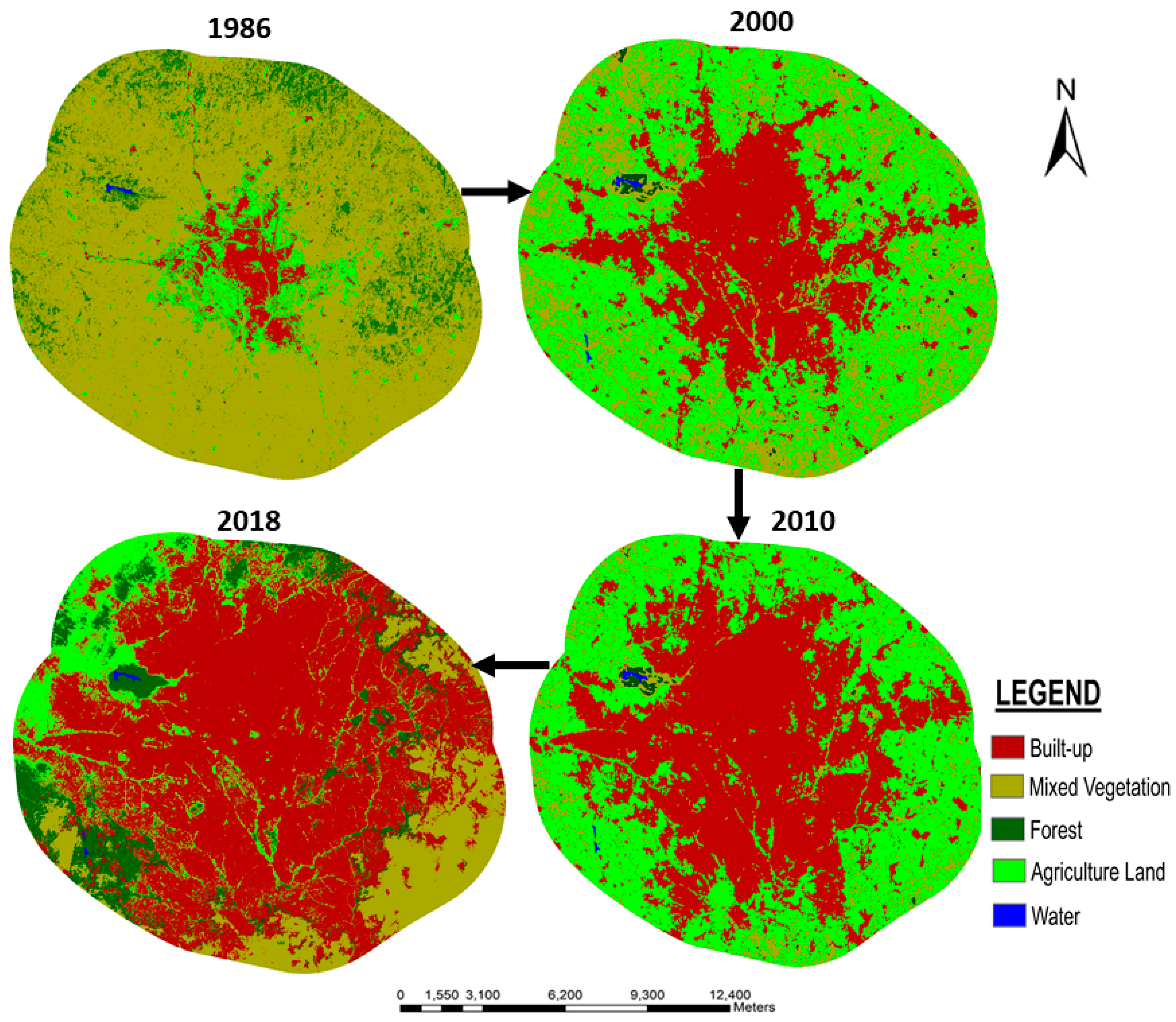
Land cover trends: At the simplest, it is the relative change in the proportion of land cover types across time. When land cover maps are available, the user can calculate the proportions of landcover, and potentially aggregate them over administrative regions to generate a picture of differing trends in urbanization, agricultural expansion, or deforestation etc. Estimates of trends of land cover change are generally important for administrative and management applications.

_{Maps showing land cover change (LCC) characteristics in Kumasi (1986–2018) (Source)}

Seasonal/Annual Trends: Whereas land cover change can be considered a ‘discrete’ change in the state of a pixel or parcel of land, many processes vary continuously across both time and space. Temperature is a good example. Time series of temperature measurements can be analyzed for both seasonal variation (i.e. minimum/maximum annual temperature) or when strung together across many years, as annual trends (i.e. climate change).

_{Temperature analysis over the study period (1970–2020) in Southwestern Ghana (Source)}

3. Methods for Change Mapping and Time Series Analysis#

Several approaches can be followed depending on the application context, for example:

Linear Models - Linear time series analysis techniques are predicated on the assumption that the underlying process changes at a constant rate. For example, assessing the annual rate of change in land surface temperature across a city. In general, this involves fitting a straight line through time series of the observations of interest and evaluating the magnitude and direction of the slope of the fit.
Nonlinear Models - Nonlinear time series models are employed when the time series cannot be adequately described by a straight line. For example, indicators of vegetation greenness usually have a strong seasonal component. Fitting a straight line through the data ignores intra-annual variations that might be important.
Harmonic Models, also termed spectral analysis or Fourier analysis, allow the decomposition of the periodic signal into a series of sinusoidal functions, each defined by unique amplitude and phase values. See this paper for an excellent example.
Breakpoint Models - Allows the automatic detection of breaks in time series data, and potentially the fitting of different linear and nonlinear models on either side of the break.

4. Time Series Analysis in GEE#

GEE has the functionality to derive both linear and harmonic trends from satellite imagery and environmental data. The techniques can be mixed and matched to model both simple trends, and to decompose complex trends into seasonal and annual components, and to detect and fit breakpoint models. For the purposes of this training, we will focus on developing estimates of simple linear trends across regions. The user is directed to documentation on CCDC for a more complex treatment of harmonic time series components for land cover mapping, and to LandTrendr for utilizing breakpoints for detecting landcover change. We will follow the steps below:

Identify and collect a time series of interest,
Find a location of interest, extract a time series and plot a chart,
Export the chart in excel, and fit a linear trend to it,
Fit linear trends to all pixels in the area of interest to assess rates of change.

_{Example chart of time series NDVI data from MODIS plotted in GEE from 2010 to 2019. (Source)}

5. Exercises#

5.1 Extracting and exploring time series

In this example, we will use GEE to extract a single time series from an ImageCollection and will open it in Microsoft Excel (or software of your choice). We will manually fit a linear trendline to this time series and extract the slope.
If needed, use this script to refresh your skills in finding, filtering, and clipping images,
Copy the script Time Series Analysis Example and paste into GEE editor,
Variables ST_DATE and EN_DATE specify the start and end dates,
Variable MOD13Q1 is the MODIS 16-day 500m Global NDVI/EVI product
Variable imgNDV filters all MODIS Data to get NDVI images and clip them to the region of interest.
Variable imgPET similarly filters all MOD16A2 Data to get PET images and clip them to the region of interest.
The print statements let you inspect the contents of these image collecetions in the console.
On the charts generated in the console, click on the upper right corner to open the chart in a new window.
Download the chart as a CSV sheet by clicking on the button in the upper right corner.
Open this CSV in Microsoft Excel and fit a trendline to it.
Please complete Exercise 1
Please submit your exercise here

5.2 Conducting linear time series analyses across large regions

In this example, we will fit linear trends to all pixels across a large region and will assess how trends vary geographically for different parameters.
Copy the script Linear Time Series Fitting and paste into GEE editor,
Variables ST_DATE and EN_DATE specify the start and end dates,
Function createTimeBand adds a ‘time band’ to any image. Think of this as adding the date column to your excel sheet. This will form the X-axis.
Variables ERA5_temp and ERA5_rain collect ERA5 reanalysis climatological data, filter dates set above, clip them to the region of interest, and add the time band.
Variable linearFitTemp fits the linear fitting ‘reducer’ to the stack of images. A ‘reducer’ is a function that takes information from all bands and computes a certain metric from it. Common reducers include mean, median, min, and max. The linearFit reducer fits a linear regression model for every stack of pixels against the time band, and outputs the scale (slope), and the offset (intercept) of the fitting line.
Inspect the respective histograms to find the best visualization parameters for the map displayed.
Please complete Exercise 2
Please submit your exercise here

6. What’s Next?#

Module 2 - Change Detection